neuron.ai

Understanding Transformers - Attention Is All You Need explained

This post is the first part of our new series Understanding AI. In this series, we explain important papers in the field of Artificial Intelligence using easily understandable explanations and great visualizations. We begin this series by describing the paper Attention Is All You Need [1] published by Ashish Vaswani et al. of Google Brain and Google Research in 2017 in which the Transformer architecture was proposed.

1. Introduction

In machine learning, Recurrent Neural Networks (RNNs) and Long Short-Term Memory (LSTM) networks have been and are often still used for processing sequential data. Even though they were state of the art just a few years ago their performance is vastly limited. Since both methods process one sample sequentially, the training is very time-intensive. In the case of the sample being a sentence, these methods would process it word by word (or more precisely, token by token). This recurrent processing leads to these methods forgetting about the parts at the beginning of the sequence and only remembering the last few parts it just processed. This is another reason why the performance of these methods is limited, especially when dealing with long sequences. In this post, the amount of the previously processed parts of a sequence a model or mechanism remembers is referred to as reference window. In practice, due to the “forgetting” of previous inputs of a sequence, the reference windows of RNNs and LSTM networks are (very) limited. The attention mechanism solves both problems. It has an infinite reference window (does not “forget” previous inputs / does not suffer from short-term memory) and reduces the number of computation steps and the training time significantly by not processing sequences sequentially while training.
In the paper “Attention Is All You Need”, [1] Ashish Vaswani et al. of Google Brain and Google Research propose an architecture which is called the Transformer. It is the first transduction model using only the attention mechanism without using sequence-aligned RNNs or convolution. Transformers are used in many different fields, for example in life sciences to generate new protein sequences or in natural language processing (NLP) for applications like translation and next-word prediction. In this post, for simplicity, we assume that our input are sequences of words (sentences). Additionally, we assume that we use the Transformer for a sequence-to-sequence (seq2seq) task. Throughout this post, information and (edited) visualizations from [1, 2] are presented.

2. Attention

In the field of machine learning, the focus between parts of the inputs is referred to as attention. In the case of the input being sentences, attention values represent the focus between the different words of the sentences. More accurately, they represent the focus between the tokens of the sentences. In NLP, tokens are the smallest unit of text that are meaningful for analysis, usually individual subwords. This means that the attention mechanism highlights some parts of the input data while it diminishes other parts. After embedding the input tokens (converting the tokens to high-dimensional vectors of numerical values) using learned embeddings we forward the result through three different linear layers to obtain the queries, keys and values which are then used to calculate the attention values. The key, value and query concept is analogous to retrieval systems. For example, when you search for videos on YouTube, the search engine will map your query (text in the search bar) against a set of keys (video title, description, etc.) associated with candidate videos in their database and then present you the best-matched videos (values). Similarly, in the attention mechanism, the values can be thought of as the interesting things about the source sentence, the keys as the way to index the values and the queries as the features the mechanism is interested in.

2.1. Scaled Dot-Product Attention

The two most commonly used attention functions are additive attention [4] and dot-product (multiplicative) attention. Additive attention computes the compatibility function using a feed-forward network with a single hidden layer. While the two are similar in theoretical complexity, dot-product attention is much faster and more space-efficient in practice, since it can be implemented using highly optimized matrix multiplication code. The attention the authors chose is a scaled version of the dot-product attention.
Once we obtain our key, query and value vectors by forwarding our embedded input through three different linear layers, the scaled dot-product attention is computed. As illustrated in Figure 1, the attention weights get calculated by taking the dot-product of the queries and the keys, dividing it by the square root of the dimension of the keys and putting the resulting matrix into the softmax function. Without the scaling, the dot products could grow large in magnitude if we have large values for the dimension of the keys. This would push the softmax function into regions where it has extremely small gradients.

Once we obtain our key, query and value vectors by forwarding our embedded input through three different linear layers, the scaled dot-product attention is computed. As illustrated in Figure 1, the attention weights get calculated by taking the dot-product of the queries and the keys, dividing it by the square root of the dimension of the keys and putting the resulting matrix into the softmax function. Without the scaling, the dot products could grow large in magnitude if we have large values for the dimension of the keys. This would push the softmax function into regions where it has extremely small gradients.

Short explanation: To better understand why the scaling is necessary, take two simple two-by-two matrices with 1s on one diagonal and -1s on the other. These matrices have a mean of 0 but a variance of 1. If we take the dot-product of these two matrices, we get a matrix with 2s on one diagonal and -2 on the other. Therefore, this matrix still has a mean of 0 but a variance of 2. This means that the variance of the dot-product can be very high if we have keys and queries with very large dimensions.

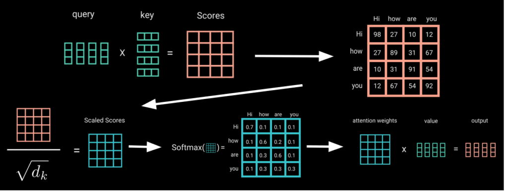
Illustration of calculating the Scaled Dot-Product Attention
Figure 1: Scaled Dot-Product Attention.
By taking the dot-product of the attention weights and the values one gets the scaled dot-product attention. Figure 2 illustrates the process of calculating scaled dot-product attention in more detail. If the attention gets calculated between the same input as visualized in Figure 2, it is called self-attention.
Scaled Dot-Product Attention Detailed Overview
Figure 2: Calculating the Scaled Dot-Product Attention.

2.2. Multi-Head Attention

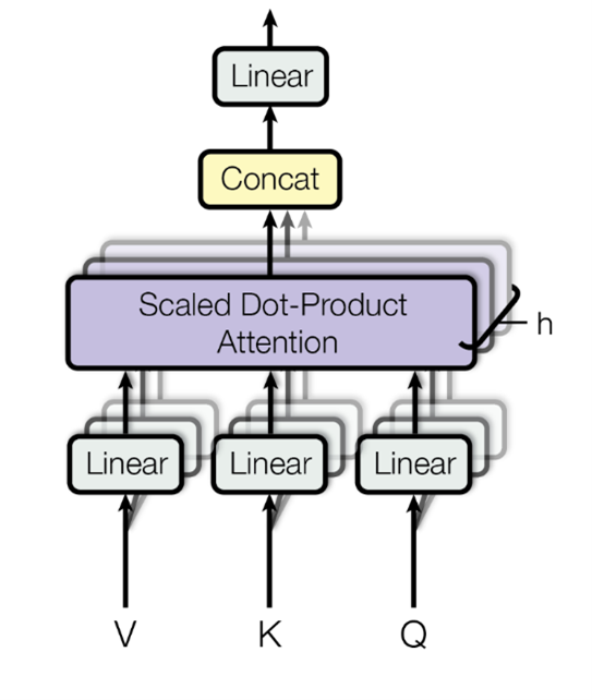
Instead of performing a single attention function with one key, value and query vector, the embedded input tokens are linearly projected h times with different, learned linear projections to obtain h heads each consisting of different value, key and query vectors.
In the paper, the authors used a value of 8 for h. Afterward, as visualized in Figure 3, the attention function is performed on each of these heads in parallel. Finally, the outputs of the heads are concatenated and passed through a linear layer. The idea behind Multi-Head Attention is to have different heads which can interpret completely different relationships between words. Note that after concatenating, the output vector consists of data from h different heads and the linear layer then “mixes” the data of all the heads. In Figure 4 different interpreted relationships of two heads are visualized.
Multi-Head Attention
Figure 3: Multi-Head Attention consists of several attention layers running in parallel.
Two heads which learned different relationships between the words.
Figure 4: Two heads which learned different relationships between the words.

3. Input and Output Embedding

To convert the input tokens and output tokens to vectors of a certain dimension, the authors used learned embeddings. In the proposed model, the same weight matrix is shared between the input and output embedding layers. These weights are multiplied in the embedding layers by the square root of the dimension of the output vector of the embedding.

4. Positional Encoding

Due to the fact that Transformers do not use recurrence, information about the positions must be added to the embedding. This is done using positional encodings where the sine function is used in even time steps and the cosine function is used in uneven time steps for creating a vector that is added to our input or output embedding vector. The input to Equations 1 and 2 is the position pos and the dimension i as detailed below.

Positional Encoding Equations
Equation 1 and 2: Positional Encoding Equations.

The authors chose these functions because they hypothesized that it would allow the model to easily learn to attend by relative positions, since for any fixed offset k, PE(pos+k) can be represented as a linear function of PE(pos).

5. Structure of a Transformer

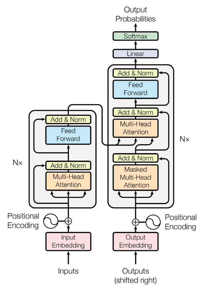
As visualized in Figure 5, a Transformer consists, in addition to input and output embeddings and a positional encoding, of an encoder and decoder. The encoder discovers interesting relationships between the words of the source sentence, whereas the decoder generates the wanted output text sequence.
Architecture of a Transformer
Figure 5: Architecture of a Transformer.

5.1. Encoder

The encoder is composed of a stack of N=6 identical layers (one after another). Each layer consists of two sub-layers, which are a Multi-Head Attention block and a fully-connected feed-forward network with two linear transformations. Around each sub-layer, a residual connection and a layer normalization are employed. This means that for each sub-layer the input is added to the output of the sub-layer and the result gets normalized. This enhances the backward gradient flow through the different layers of the model. To be able to use residual connections around each sub-layer, the dimension of the outputs of the different sub-layers has to stay the same. The authors chose a dimension of 512.

5.2. Decoder

As visualized in Figure 5, the decoder has a very similar architecture. It has a Multi-Head Attention block and a small neural network, too. Additionally, the decoder includes a Masked Multi-Head Attention block which is placed before the two other sub-layers.

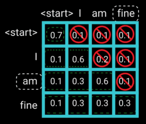
As the name suggests, the Masked Multi-Head Attention block involves a look-ahead mask that prevents the Transformer in the time step t to obtain information about relationships to words after time step t when training. To be more precise, the mask is applied to the target sequences the Transformer gets trained on. Without this mask, information about the sentence, word or label we want to predict would be available during the forward pass while training the Transformer. Figure 6 illustrates which values should be masked by using “I am fine” as an example input. If we want to predict the next word after “am”, we should not have information about the next word(s) which in this case would be “fine”.
Masked Self-Attention
Figure 6: Masked Self-Attention.

This mask consists of zeros in indices where it should not block the information as well as minus infinity in indices where it should block it. To prevent the information we want to block to pass, we add the look-ahead mask directly after scaling the dot product of the queries and keys. After the mask is added, the softmax function of the resulting matrix is taken, which turns the minus infinity values into zeros. This leads to the wanted result, i.e., it ensures that the predictions for time step t can depend only on the known outputs with time step smaller equal than t This process is illustrated in Figure 7.

Masking Process
Figure 7: Illustration of the Masking Process.
Since we know our target sequences while training, we can apply different masks for the corresponding time steps across the time dimension of one tensor at once. Therefore, one sequence only needs one forward pass through the encoder and decoder. This means that the Transformer is not auto-regressive while training (= does not consume its previously generated outputs as additional input when generating the next output) which results in a significantly shorter training time. However, at inference, since we do not know the target sequences and one output of the encoder is calculated using the previous ones, the Transformer is not auto-regressive.
As in the encoder, there are residual connections around each of the sub-layers also in the decoder. Additionally, note that the output of the encoder, the keys and values which contain the attention information, are part of the input to the second sub-layer of the decoder. While we get the keys and values for the decoder from the encoder, the queries for the decoder are the outputs of the first block of the decoder, which is the masked multi-head attention block.

5.3. Applications of Attention

The Transformer has three different applications of multi-head attention as visualized in Figure 8. In the encoder, the attention used is defined as self-attention since it learns the attention weights between the input itself. In the first attention block of the decoder, we use masked attention, which is a self-attention with a look-ahead mask to (as explained in the section about the decoder) prevent the Transformer from obtaining information about the next time steps. The last application of attention is in the second attention block of the decoder. This application is called the encoder-decoder attention since it uses data from the encoder and decoder. To be more precise, the output of the masked attention block are the queries and the output of the encoder are the values and keys for this attention block.
Applications of Attention
Figure 8: Applications of Attention.

5.4. Linear Classifier

After the input passes the encoder and decoder it reaches the classifier. While the proposed classifier is just a single linear layer, it can be modified or extended by, for example, adding multiple attention blocks or linear layers and the dimension of the output of the classifier depends on the specific task. To get the probability distribution, the softmax function is used once again. Finally, at inference, the look-ahead mask is updated for the next time step.

6. Training

For training the Transformer, the authors used the Adam optimizer and a learning rate scheduler with a warm-up phase. In this warm-up phase (which lasts for 4000 steps) the learning rate increases linearly as can be seen in Equation 3.
Learning Rate Equation
Equation 3: Learning Rate Scheduler.
The authors apply dropout to the output of each sub-layer before it is added to the sub-layer input and normalized. In addition, they apply dropout to the sums of the embeddings and positional encodings in both the encoder and decoder stacks. For the base model, they use a dropout rate of 0.1. Furthermore, during training, they employed label smoothing with ε=0.1 to make sure that the Transformer learns to be more unsure of its decisions. The hardware used for training consisted of 8 NVIDIA P100 GPUs.

7. Results

The authors of the paper detailed the performance on the task of machine translation of one base model trained for 100 000 steps and 12 hours and one big model trained for 300 000 steps and 3.5 days on two datasets. The datasets they used are the datasets for the WMT 2014 English-to-German and English-to-French translation tasks with 4.5 million and 36 million sentence pairs, respectively. Furthermore, they consist of 37 000 and 32 000 tokens, respectively. Both models outperform the best previously reported model at the English-to-German translation task. The big model additionally outperforms every reported single model with one-fourth of the training cost of the best previously reported model.

8. Conclusion

The Transformer architecture already displaced many RNNs and LSTM networks. Vision Transformers as proposed in the paper “An Image is Worth 16×16 Words: Transformers for Image Recognition at Scale” [3] are being increasingly used instead of CNN’s, especially when using a very large dataset. It clearly is the new state of the art. Examples of Transformers include BERT, GPT-3 and GPT-4.
Many applications of Transformers clearly show that they are more capable than previous methods involving recurrence and/or convolution. Due to the unlimited reference window and non-sequential processing Transformers outperform other known architectures in capability and speed.
However, Transformers need a very large training dataset or even multiple datasets (possibly from different sources) for them to perform well. Additionally, another limitation of the attention mechanism is that the amount of weights used grows quadratically with the length of the sequences. Training Transformers is only possible due to the architecture of modern GPUs and their support for parallel operations.

The success of the attention mechanism and Transformer indicate that it probably will be the foundation for many successful architectures in the future.

Thank you for your Attention! 😉

Tobias Morocutti

Tobias Morocutti studies Artificial Intelligence at Johannes Kepler University (JKU) in Linz. He currently is in the last semester of his Bachelor programme and works at the Institute of Computational Perception at JKU where he specializes on Audio Processing and Machine Learning. In 2022, before working at the Institute of Computational Perception, he participated at Task 1 (Low-Complexity Acoustic Scene Classification) of the annual DCASE challenge where he ranked third. This year he participates at the same challenge with his work colleagues. In addition to Audio Processing and Machine Learning in general, Tobias is also very interested in Computer Vision.

References

[1] A. Vaswani, N. Shazeer, N. Parmar, J. Uszkoreit, L. Jones, A. N. Gomez, L. Kaiser, and I. Polosukhin, “Attention is all you need”, CoRR, vol. abs/1706.03762, 2017. [Online]. Available: http://arxiv.org/abs/1706.03762

[2] M. Phi, “Illustrated guide to transformers neural network: A step by step explanation”, 2020. [Online]. Available: https://www.youtube.com/watch?v=4Bdc55j80l8

[3] A. Dosovitskiy, L. Beyer, A. Kolesnikov, D. Weissenborn, X. Zhai, T. Unterthiner, M. Dehghani,M. Minderer, G. Heigold, S. Gelly, J. Uszkoreit, and N. Houlsby, “An image is worth 16×16 words: Transformers for image recognition at scale”, 2021.

[4] D. Bahdanau, K. Cho, and Y. Bengio, “Neural Machine Translation by Jointly Learning to Align and Translate”, 2016